Cooling Curves and its Types, Construction of Phase Diagrams

 Cooling curves are obtained by plotting the measured temperatures at equal intervals during the cooling period of a melt to a solid.

COOLING CURVES

(Time-Temperature Cooling Curves)

✓ Cooling curves are obtained by plotting the measured temperatures at equal intervals during the cooling period of a melt to a solid.

✓ The data obtained from these cooling curves are useful in constructing the equilibrium diagram.

1. Types of Cooling Curves

Three main types of cooling curves are shown in Fig.1.9.

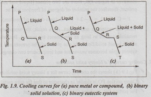
1. Cooling curve for pure metal or compound

✓ Fig.1.9 (a) shows the cooling curve for a pure metal or a compound.

✓ From P to Q, the curve proceeds at a uniform rate and at point Q, the first crystals begin to form.

✓ As solidification proceeds, the latent heat of fusion is liberated in such amount that the temperature remains constant from Q to R until whole mass has entirely solidified. The period QR is known as the horizontal thermal arrest.

✓ Further cooling from point R will cause the temperature to drop along curve RS. The slopes of PQ and RS curves depend upon the specific heats of liquid and solid metals respectively.

✓ In the region PQ, only liquid phase is present while in the region RS only solid phase is present.

Applying Gibb's condensed phase rule, we get

F = C - P + 1 = 1 - 1 + 1 = 1 (one degree of freedom)

Thus the temperature can be varied independently without altering the equilibrium.

✓ However in region QR, there are two phases (liquid and solid) present, therefore the number of degrees of freedom will be

F = C - P + 1 = 1 - 2 + 1 = 0 (zero degree of freedom) 

Thus, the system is non-variant. As a result, the temperature remains constant as long as two phases are present. But when all the liquid solidifies, only one phase will be present and the system again becomes univariant and temperature can change.

2. Cooling curve of a binary solid solution

✓ Fig.1.9 (b) shows the cooling curve for a binary solid solution. 

✓ Curve portion PQ is similar in character to that for pure metal. 

✓ For portion QR, applying Gibb's phase rule, we get

F = C - P + 1 = 2 - 2 + 1 = 1 (one degree of freedom)

Thus the system is univariant and the temperature will change during solidification. 

✓ The slope of the cooling curve will change due to the evolution of latent heat of crystallisation.

✓ Beyond point R, there will be only solid phase and the of Ontemperature falls along line RS.

3. Cooling curve of a binary eutectic system

✓ Fig.1.9 (c) shows the cooling curve for a binary eutectic gorb of system.

✓ A binary eutectic system (or a multiphase alloy) has two components that are completely soluble in the liquid state but entirely insoluble in the solid state.

✓ The system is liquid along PQ upto point Q.

✓ At point Q, the temperature drops along QR and crystallization of one component starts.

✓ At point R, the liquid composition reaches such a level that two components crystallise simultaneously from the solution and the temperature remains constant until all the liquid solidifies. This is known as the eutectic reaction.

✓ Thus eutectic reaction can be defined as the transformation, during cooling, of a liquid phase isothermally and reversibly into two solid phases.

✓ The cooling from S to T is as usual.

 

CONSTRUCTION OF PHASE DIAGRAMS

✓ The construction of the phase diagram for a binary solid solution (such as Cu-Ni) from series of liquid-solid cooling curves is illustrated in Fig. 1.10.

✔ If two metals of a binary solid solution (such as Cu-Ni) system are mixed in different compositions, melted and then cooled, and a cooling curve can be constructed for each composition, as shown in Fig.1.10 (a).

The cooling curves for pure metals show horizontal thermal arrests at their freezing points, as shown for pure copper and nickel in Fig.1.10 (a) at AB and CD.

✓ Binary solid solutions exhibit slope changes in their cooling curves at the liquidus and solidus lines, as shown in Fig.1.10 (a), at compositions of 80% Cu - 20% Ni, 50% Cu - 50% Ni, and 20% Cu - 80% Ni.

✓ The slope changes at L1, L2, and L3 in Fig. 1.10 (a) correspond to the liquidus points L1, L2, and L3 of Fig.1.10 (b). Similarly, the slope changes at S1, S2, and S3 of Fig. 1.10 (a) corresponds to the points S1, S2, and S3 on the solidus line of Fig.1.10 (b).

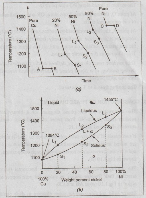
Fig. 1.10. Construction of the Cu-Ni equilibrium phase diagram from liquid-solid cooling curves.

(a) Cooling curves, and (b) Equilibrium phase diagram

✓ Thus the constructed phase diagram for Cu-Ni system from the cooling curves is shown in Fig. 1.10 (b).

Note 

1. Liquidus: In a phase diagram, the line above which only a liquid phase is present, is known as liquidus. The liquidus line separates liquid and liquid + solid phase regions.

2. Solidus: In a phase diagram, the line below which only a solid phase is present, is known as solidus.