Transverse loading on beams

 Beam is a structural member which is supported along the length and subjected to external forces or loads acting transversely i.e., perpendicular to the centre line.

Chapter - 2

TRANSVERSE LOADING ON BEAMS AND STRESSES IN BEAM

• Beams

• Types of Supports

• Types of Load

• Shear Force and Bending Moment

• Relationship between Shear Force and Bending Moment

• Shear Force and Bending Moment Diagrams

• Theory of Simple Bending

• Load carrying Capacity

• Flitched Beams

• Shear Stresses in Beams

• Solved Problems

• Solved University Problems

• Two Mark Questions and Answers

1. BEAMS

Beam is a structural member which is supported along the length and subjected to external forces or loads acting transversely i.e., perpendicular to the centre line. Beam is sufficiently long when compared to the lateral dimensions.

1. TYPES OF BEAMS

The following are the important types of beams.

(a) Cantilever beam

(b) Simply supported beam

(c) Overhanging beam

(d) Fixed beam and

(e) Continuous beam

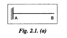
(a) Cantilever beam

A beam with one end free and the other end fixed is called cantilever beam. Refer Fig.2.1(a).

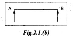
(b) Simply supported beam (SSB)

A beam supported or resting freely on the supports at its both ends is called SSB. It is shown in Fig.2.1(b).

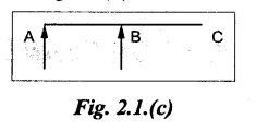
(c) Overhanging beam

If the one or both the end portions are extended beyond the support, then it is called overhanging beam. Refer Fig.2.1(c).

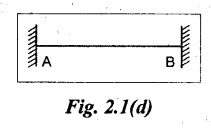
(d) Fixed beam

A beam whose both ends are fixed or built into the walls, is called fixed beam. Refer Fig.2.1(d).

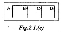
(e) Continuous beam

A beam which has more than two supports is called continuous beam. Refer Fig.2.1(e).

2. TRANSVERSE LOADING ON BEAMS

A load which is acting vertically downward on the horizontal beam is called Transverse load.

3. TYPES OF TRANSVERSE LOAD

A beam may be subjected to the following types of loads.

(a) Point or Concentrated Load

(b) Uniformly Distributed Load (UDL)

(c) Uniformly Varying Load (UVL)

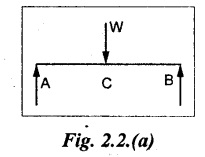
(a) Point or Concentrated Load

A load (W) which is acting at a particular point is called point load. Refer Fig.2.2(a).

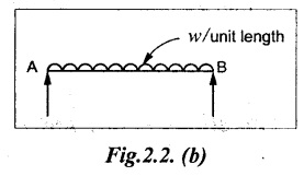
(b) Uniformly Distributed Load (UDL)

A load which is spread over a beam in such a manner that the rate of loading 'w' is uniform throughout the length.

Note

For solving problem, the UDL is converted into a point load, acting at the center of the UDL.

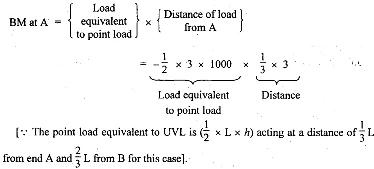
(c) Uniformly Varying Load (UVL)

A load which is spread over a beam in such a manner that the rate of loading uniformly varies from point to point along the beam. The load is zero at one end and increases uniformly to the other end. It is also called as triangular load.

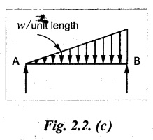
Note

For solving problems on this, the total load is assumed to be acting at a distance of 2/3 of the total length of the beam from the zero end (in fig left end) or 1/3 of the total length of the beam from the maximum load end (in fig right end).

4. SHEAR FORCE AND BENDING MOMENT

Shear Force (SF)

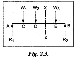
Shear Force (SF) at a cross section is the algebraic sum of the forces acting on one side of the section or the other. The sum of those forces to the left of XX axis is numerically equal but in opposite direction to the sum of those to the right. Since the resultant force acting on a beam must be zero. Shear force may also be defined as the unbalanced vertical force to the right or left side of the section.

Bending Moment (BM)

Bending Moment (BM) at a cross section is defined as the algebraic sum of the moments of all the forces acting on any one side of that section. The moment obtained by the forces on the left of the beam will be numerically equal and opposite to the right of the beam.

5. SIGN CONVERSIONS FOR SHEAR FORCE AND BENDING MOMENT

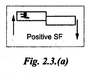
(i) Shear Force

If the external loads on the left of the section are acting 'upward' or right portion 'downward', it is called positive Positive shear force. Refer Fig.2.3(a).

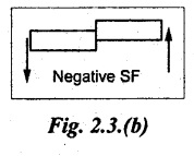
If the loads on the left portion are acting downward or right portion to upward is called Negative shear force. Refer Fig.2.3(b).

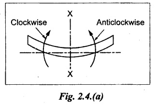
(ii) Bending Moment

Bending moment is said to be positive or sagging, if the moment of the force in the left side of the beam is clockwise or right side of the beam is counter clockwise. Otherwise, the beam tends to bend in a concave manner. Refer Fig.2.4(a).

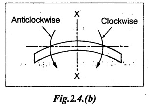
Bending moment is said to be negative or hogging, if the moment of the force in the left side of the beam is counter clockwise or right side of the beam is clockwise. Otherwise, the beam tends to bend like convex manner. Refer Fig.2.4(b).

6. RELATION BETWEEN SF AND BM

Shear force and Bending moment will be different at different cross-section. depending upon the loading on the beam. The variation in their values can be shown graphically by plotting the SF and BM as ordinates against positions of cross sections as x axis. Positive and negative values are plotted on opposite sides of the base line. These diagrams are known as the shear force diagram and bending moment diagram.

Consider, a beam carrying a UDL of w per unit length. Now consider an element of the beam between two cross sections A and B at a distance of dx apart. Let F and (F + dF) are the shear forces at A and B, M and (M + dM) are the bending moments at A and B respectively.

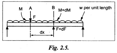
For equilibrium condition, the algebraic sum of the vertical forces is equal to zero.

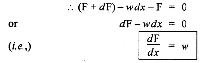
From above relation, it is obvious that the rate of change of SF which is the rate of loading per unit length of the beam.

Similarly, taking moments of forces and couples about B, ΣM = 0.

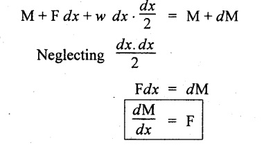
From the above relation, the rate of change of BM is equal to the SF at that section.

Note

For maximum value of BM, dM/dx = 0. But dM/dx = F, therefore the BM is maximum at a section where SF is zero or changes its sign.

7. IMPORTANT POINTS FOR CALCULATING SF AND BM

(a) Points for calculating SF

✔ Consider any cross section about which the SF is to be calculated.

✔ Consider all the forces (including reactions at the supports) which act either to the right or left of the section.

✔ Find the algebraic sum of the all forces and reactions by using conversion of SF. This will be the SF at that section.

(b) Points for calculating BM

✔ Consider a section about which the BM is to be calculated.

✔ Take the moment of all the forces either to the right or to the left of that section.

✔ Find the algebraic sum of these moments by using sign conversion of BM. This will be the BM at that section.

8. IMPORTANT POINTS FOR DRAWING SHEAR FORCE AND BENDING MOMENT DIAGRAMS

(a) For shear force diagram (SFD)

✔ If the point load acts vertically downward, the SFD will increase or decrease suddenly by a vertical straight line perpendicular to the base line.

✔ If load is acting between two cross sections, the SF will remain constant and the SFD will be horizontal straight line parallel to the base line.

✔ If UDL is acting on the beam, the SFD will be a slopping straight line.

✔ If UVL is acting on the beam, the SFD will be a parabolic curve.

✔ When a point load is acting in a region of UDL, the SFD will have two slopping lines separated by a vertical straight line at the point load.

✔ In a cantilever beam, the SF will have maximum value at the fixed ends. In simply supported beam, the SF will have maximum value at the supports.

(b) For bending moment diagram (BMD)

✔ The BM at the free end of the cantilever and at the two supports of the simply supported beam will be zero.

✔The BMD in a region between two point loads will be a slopping straight line. ✔ The BMD of UDL will be a parabolic curve.

✔ The BMD of UVL will be a cubic curve.

✔ In overhanging beams, the BM changes its sign or the beam changes its curvature. The point where the BM is zero or changes its sign is called point of contraflexure (or inflection).

9. NATURE OF SFD AND BMD FOR VARIOUS LOADS

1. Point load or Concentrated load

The nature of SFD and BMD will be rectangle and triangle for any type of beams respectively.

2. UDL

The nature of SFD and BMD will be triangle and parabola for any type of beams respectively.

3. Uniformly Varying Load

The nature of SFD and BMD will be parabola and cubic curve for any type of beams respectively.

10. SFD AND BMD FOR CANTILEVER BEAMS

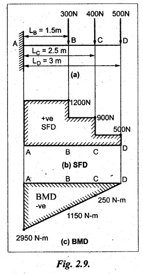
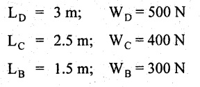
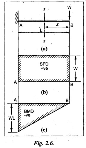
Case (a): Cantilever with single concentrated load at free end

Consider a cantilever of length L be fixed at A and free at B carrying a concentrated load W at the free end as shown in Fig.2.6(a).

Consider a cross section x-x at a distance of x from the free end B

SF calculation

SF at B = = +W (+ve due to right side downward load)

SF at X-X = +W (Because no load between B and X-X)

SF at A = +W (due to same reason as above)

SF between A and B will be constant and +ve. So, the values of SF are plotted above the base line and joined by straight line. It is shown in Fig.2.6(b).

BM calculation

The BM at any cross section is proportional to the distance of the section from the free end.

(i.e.,) Moment = Force × Distance

Bending moment at section X-X,

BM at X-X = -W × x = W x

When x = 0, BM at B = -W × 0 = 0

When x = L, BM at A = -W L

The BM at B is zero and WL at A, but negative. So, the values are plotted below the base line and joined by the inclined line. It is shown in Fig.2.6(c).

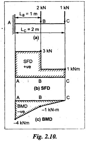
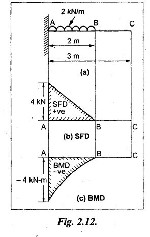
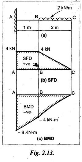
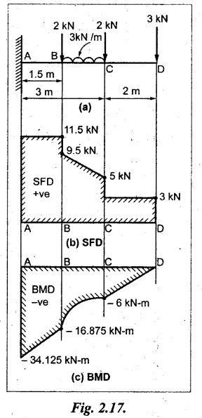
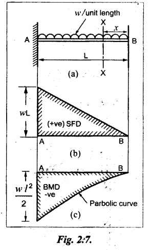
Case (b): Cantilever with UDL

Consider a cantilever of length L fixed at A and free at B carrying a UDL of w per unit length as shown in Fig.2.7(a).

Consider a section X-X at a distance x from the free end B.

SF calculation

SF at X-X,       SFx = + wx (for UDL)

when x = 0, SF at B = 0

when x = L, SF at A = + w × L

(+ve sign indicates downward load in the right side)

So, the SF linearly increases from zero at the free end to 'wL' at the fixed end. Refer Fig.2.7(b).

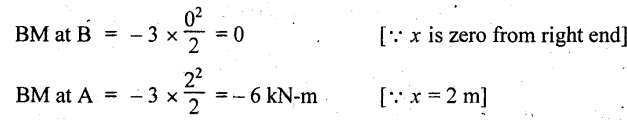
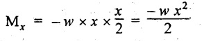
BM calculation

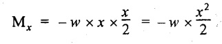
The BM at X-X,

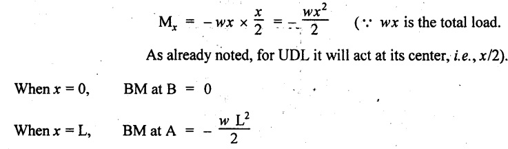
So, the BM decreases from zero at free end to  at the fixed end as shown in Fig.2.7(c).

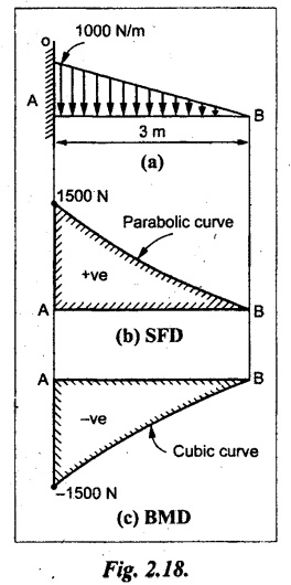
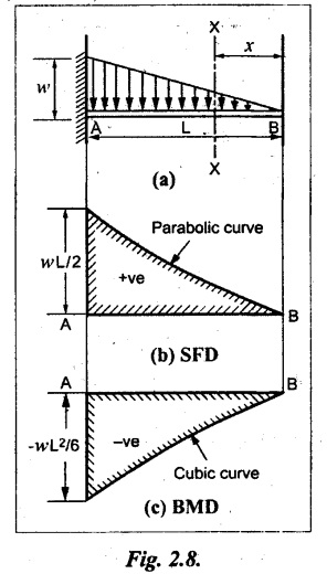
Case (c): Cantilever with Uniformly Varying Load (UVL)

Consider a cantilever of length L fixed at end A and free at B carrying a UVL from zero at the free end to w per unit length at the fixed end.

Consider the section X-X at a distance of x from the free end B.

SF Calculation

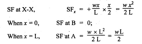
So, the SF parabolically increases from zero at the free end to wL/2 at the fixed end as shown in Fig.2.8(b).

BM calculation

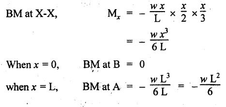
So, the BM decreases from zero at free end to  at the fixed end as shown in Fig.2.8(c).

Solved Problems On Cantilever Beams

 solved problems on cantilever beams: Transverse Loading on Beams and Stresses in Beam - Strength of Materials

SOLVED PROBLEMS ON CANTILEVER BEAMS

Example 2.1: 

A cantilever beam of length 3m carries the point loads as shown in Fig. 2.9(a). Draw the shear force and bending moment diagrams for the cantilever beam.

Given:

To draw: 

SFD and BMD

Solution:

SF calculation:

We know that, SF is the sum of forces on either left or right side of the section. Here we are considering from right side. The force acting downward and hence it is positive.

SF at D = + WD = + 500 N

SF between D and C remains constant and equal to +500 N. So, the forces are plotted above the base line and joined by the straight line.

SF at C = +WD + WC

= +500 + 400 = 900 N

SF between C and B remains constant and equal to +900 N

SF at B = +WD + WC + WB

= +500 + 400 + 300

= + 1200 N

SF between B and A remains constant and equal to +1200 N.

SF at A = + 1200 N        [since there is no load between A and B]

BM calculation

We know that,

BM at any section = Force × Distance from the corresponding section

Taking moments about the section D, C, B and A respectively from right side.

BM at D = WD × Distance from D

= -WD × 0 = 0

BM at C = -WD × Distance between D and C

= -WD × (LD - LC)

= - 500 × 0.5

= - 250 N-m

BM at B = - WD (LD - LB)- WC (LC – LB)

= - 500 × 1.5 - 400 × 1

= - 1150 N-m

BM at A = -WDLD - WC LC - WB LB

= - 500 × 3400 × 2.5 - 300 × 1.5 

= - 2950 N-m

The above result shows that the BM is zero at D and -ve value for all other points. So, the values are plotted below the base line AB and joined by inclined line.

Result:

The SF and BM values for all the points of the beam are plotted as shown in Fig.2.9(b) and (c) respectively.

Example 2.2: 

A cantilever beam of length 2m carries the point load of 1kN at its free end, and another load of 2 kN at a distance of Im from the free end. Draw the SF and BM diagrams for the cantilever beam.

Given:

LC = 2 m;

LB = 1 m;

WC = 1 kN 

WB = 2 kN

To draw: 

SFD and BMD

Solution: 

SF calculation:

SF at C = + 1 kN

SF at B = + 1 kN + 2 kN = 3 kN

SF at A = + 3 kN

BM calculation:

Taking moment from right side of the beam section considered.

BM at C = -WC × 0 = 0

BM at B = -WC (LC - LB) - WB × 0

= -1 × 1 – 2 × 0

= - 1 kN - m

BM at A = -WC × LC - WB × LB

= -1 × 2 – 2 × 1 = -4 kN - m

[Note: For details refer problem 2.1]

Result: 

SFD and BMD are represented by Fig.2.10(b) and (c) respectively.

Example 2.3:

A cantilever of length 2 m carries a UDL of 3 kN/m. Draw the SF and BM diagrams.

Given: 

L = 2 m;

w = 3 kN/m

To draw: 

SFD and BMD

Solution:

SF calculation:

We know that, for UDL,

SF at any section of the beam is given by,

SF = Load × Length of the load spread over the section

SF = 3 kN/m x Length

SF at B = 3 × 0 = 0   [ ⸪ Distance is zero at B from right end.]

SF at A = 3 kN/m × 2 m = 6 kN

For UDL, the SFD is a sloped line. Draw the SFD as shown in Fig.2.11(b). 

BM calculation:

For UDL, the BM at any section of the beam is given by,

BM = Force × Distance

BM = Load × Length of the load spreaded × Distance

(i.e.,) BM at any section x from free end is given by,

Taking moment from right side of the section considered,

BMD will be parabola for UDL. Draw the BMD as shown in Fig.2.11(c).

Result:

SFD and BMD are shown in Fig.2.11(b) and (c) respectively.

Example 2.4: 

A cantilever of length 3 m carries a UDL of 2 kN/m which run over a length of 2 m from the fixed end. Draw the SF and BM diagrams.

Given: 

L = 3 m;

w = 2 kN/m

l = 2 m.

To draw: 

SFD and BMD

Solution:

SF calculation:

SF at C = 0

SF at B = 0

SF at A = w × l = 2 kN/m × 2 m = 4 kN

Join all the values as shown in Fig.2.12(b).

BM calculation:

BM at any section x from free end is given by

Taking moment from right side of the section considered.

Join the values as shown in Fig.2.12(c).

Result: 

SFD and BMD are shown in Fig.2.12(b) and (c) respectively.

Example 2.5: 

A cantilever of length 3 m carries a UDL of 2 kN/m over a length of 2 m from the free end. Draw the SF and BM diagrams for the cantilever.

Given: 

L = 3 m;

w = 2 kN/m

l = 2 m

To draw: 

SFD and BMD

Solution:

SF calculation:

SF at C = 0

SF at B = 2 kN/m × 2 m

= 4 kN

SF at A= +4 kN

[Since, there is no load between A and B.]

The SF values between C and B are joined by a straight slopped line because of UDL and then between B and A by a straight horizontal line.

BM calculation:

BM at C = 0

Since the load is UDL, the BM values between C and B are joined by a parabolic curve. The point B and A are joined by a straight line because there is no load.

Résult:

SFD and BMD are shown in Fig.2.13(b) and (c) respectively.

Example 2.6: 

A cantilever of length 3 m carries a UDL of 3 kN/m over a whole length and a point load of 2 kN at the free end. Draw the SF and BM diagrams.

Given: 

As shown in Fig.2.14(a).

To draw: 

SFD and BMD.

Solution:

SF calculation:

SF at B = + 2 kN

SF at A = SF by point load + SF by UDL 

= +2 kN +3 kN/m × 3 m

SF at A = + 11 kN

Join all the S.F values as shown in Fig.2.14(b).

BM calculation:

BM at any section = BM by point load + BM by UDL

BM at B = 0

= -6 -13.5 = -19.5 kN-m

Draw the BM diagram as shown in Fig.2.14(b) and (c).

Result: SFD and BMD are shown in Fig.2.14(b) and (c) respectively.

Example 2: 

A cantilever of length 4 m carries a UDL of 3 kN/m run over the whole length and two point loads of 4 kN and 2.5 kN are placed Im and 2m respectively from the fixed end. Draw the SF and BM diagrams.

Given: 

As shown in Fig.2.15(a).

To draw: 

SFD and BMD

Solution:

SF calculation:

SF at D= 0

SF at C (without point load at C) = 3 kN/m × 2 m = 6 kN

Total SF at C = SF by point load

(i.e., 2.5 kN) + SF by UDL of length between C and D

(i.e., 2 m)         2.5 kN + 3 kN/m × 2 m = +8.5 kN

Similarly, SF at B (without point load at B).

= 2.5 kN +3 kN/m × 3 m = 11.5 kN

Total SF at B = +4 kN + 2.5 kN + 3 kN/m × 3 m 

= +15.5 kN

SF at A = 4 kN +2.5 kN + 3 kN/m × 4 = +18.5 kN

BM calculation:

BM at D = 0

Draw the SF and BM diagrams as shown in Fig.2.15(b) & (c).

Result: 

SFD and BMD are shown in Fig.2.15(b) & (c) respectively.

Example 2.8:

A cantilever of 3m long carries a UDL of 12 kN/m is spread over a length of 1.5m from the free end. It also carries a point load of 15 kN at free end and another point load of 8 kN at 1 m from the fixed end. Draw the SFD and BMD.

Given: 

As shown in Fig.2.16(a).

To draw: 

SFD and BMD

Solution:

SF calculation:

SF at D = +15 kN

SF at C = +15 kN + 12 kN/m × 1.5 m

= +15 + 18 = +33 kN

SF at B = +15 kN + 12 kN/m × 1.5 m + 8 kN

= +41 kN

SF at A = +41 kN

SF values between C and D are joined by a straight inclined line because of UDL acting at that section.

BM calculation:

BM at D = 0

BM at C = BM by point load at D + BM by UDL

The BM values between C and D are joined by parabolic curve. Since, the load is UDL. The BM values between BC and AB are joined by a straight inclined line. Thus, the BM is obtained.

Result: 

The BMD and SFD are shown in Fig.2.16(b) & (c) respectively.

Example 2.9: 

A cantilever beam of length 5m is loaded as shown in Fig.2.17(a). Draw the SF and BM diagrams.

Given: 

As showin Fig.2.17(a).

To draw: 

SFD and BMD

Solution:

SF calculation:

SF at D = 3 kN

SF at C = 3 + 2 = + 5 kN

SF at B (without point load)

= 3 kN + 2 kN + 3 kN/m × 1.5 m = + 9.5 kN

Total SF at B (i.e., considering point load)

3 kN + 2 kN + 3 kN/m × 1.5 + 2 kN = +11.5 kN 

SF at A = +11.5 kN

Draw the SF diagram as shown in Fig.2.17(b).

BM calculation:

BM at D = 0

The BM values between B and C are joined by parabolic curve because of UDL and all other values are joined by straight inclined lines as shown in Fig.2.17(c).

Result: 

BMD and SFD are shown in Fig.2.17(b) & (c) respectively.

Example 2.10: 

A cantilever beam 3m long carries a gradually varying load, zero at the free end to 1000 N/m at the fixed end. Draw the SF and BM diagrams for the beam.

Given: 

As shown in Fig.2.18(a).

To draw: 

SFD and BMD

Solution: 

SF calculation:

SF at B = 0.

SF at A = Area of the triangle ABO

1/2 × 3 × 1000 = 1500 N

The SF is zero at B and increases parabolically to 1500 N at A.

BM calculation:

BM at B = 0

Draw the cubic curve between A and B as shown in Fig.2.18(c).

Result: 

The SFD and BMD are shown in Fig.2.18(b) & (c) respectively.