Boundary Layer Concepts

 During a fluid flow, layer of fluid which comes in contact with the boundary surface of solids body and adheres to it due to viscosity.

BOUNDARY LAYER CONCEPTS

1. Introduction

During a fluid flow, layer of fluid which comes in contact with the boundary surface of solids body and adheres to it due to viscosity. Viscosity is the of the most important property of fluid. The neglect of viscosity in fluid flow problems gives solutions in which are not applicable in real flow situations. In all real fluids flow cases the consideration of viscosity is important. However, the inclusion of viscosity in the equation of motion makes them non linear and almost impossible for obtaining exact solutions. In the year 1904, a German scientist named Ludwig prandtl had shown that the effect of viscosity can be confined to a thin layer near the boundary (solid body (or) flow pipes) is called boundary layer and the flow outside of this boundary layer can be treated as potential flow.

2. Boundary Layer

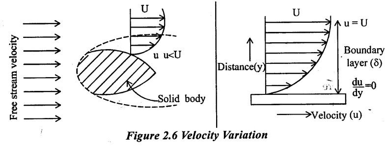
During a real fluid flow in the solid body surface, layer of fluid which comes in contact, with the boundary surface adheres to it due to viscosity. Hence this layer attains the same velocity as that of the solid boundary surface. If there is no slippage between them. If the solid boundary surface is stationary the fluid layer of boundary surface will have zero velocity. The other fluid layer adjacent to the stationary boundary undergo retardation from the top surface. A small fluid region in the immediate vicinity of the boundary surface is developed in which the velocity of flowing fluid increases gradually from zero of the solid boundary surface to the velocity of the steady stream (or) free stream air velocity (U) and as a result velocity gradient du/dy will exists to the narrow region of the fluid in which the variation of dy velocity from zero to free steam velocity in a direction normal to the boundary takes place is called boundary layer. The term boundary layer is used to describe the thin layer of fluid flow on the boundary surface within which the shear stresses are of appreciable magnitude.

Outside the boundary layer, the velocity of the fluid is same as the main stream. Hence there is no shear stress acting and velocity gradient does not exists that region. The effect of boundary layers are (i) It adds on to effective thickness of the solid body which is called displacement thickness, there by increasing the pressure drag on the soild body (ii) As velocity gradient exists in the boundary layer, shear force acts on the boundary surface, resulting in skin friction drag.

3. Boundary Layer Theory

The theory dealing with boundary layer is called boundary layer theory. According to this theory the flow of fluid in the neighbour hood of the solid boundary is divided into the two parts shown in fig 2.6

(i) A very thin layer of the fluid, called boundary layer, near solid boundary the velocity varies from zero to free stream velocity(U). In this region the velocity gradient du/dy (u is the fluid velocity in x- direction and y is perpendicular distance dy from the boundary surface.) varies with y and it has high values close to the boundary. This high velocity gradient gives rise to large shear stress at the boundary surface.

(ii) The remaining fluid outside boundary layer constant velocity equal to free stream velocity and has no shear stress.

Applications:

(i) It is very important in many problems of aerodynamics, because it is directly responsible for the drag experienced by a body immersed in a fluid.

(ii) In design of an aircraft, more concentration is given on controlling the behavior of the boundary layer, to minimize drag.

4. Effect of Boundary Layer

(i) Boundary layer add the effective thickness of the body through the displacement thickness hence increase in the pressure drag

(ii) The shear force at the boundary surface create the skin friction drag

5. Factors affecting the Boundary Layer

Following are the various factors which influence the growth of boundary layer on a smooth flat plate are as follows.

(i) The distance 'X' from the leading edge:

It various directly with distance 'X'. More the distance 'X' the thickness of boundary layer is also more

(ii) Free stream velocity:(U)

Boundary layers varies inversely as the free stream velocity U. If free stream velocity increases, thickness of boundary layer decreases and vice-versa. 

(iii) Viscosity of fluid: (μ)

Boundary layer varies directly with viscosity. If viscosity of fluid is more, the thickness of boundary layer is more and vice-versa.

(iv) Density of fluid: (ρ)

Boundary layer varies inversely with density for lower density fluid, thickness of boundary layer is more and vice-versa.

6. Boundary Layer Development Over a Flat Plate

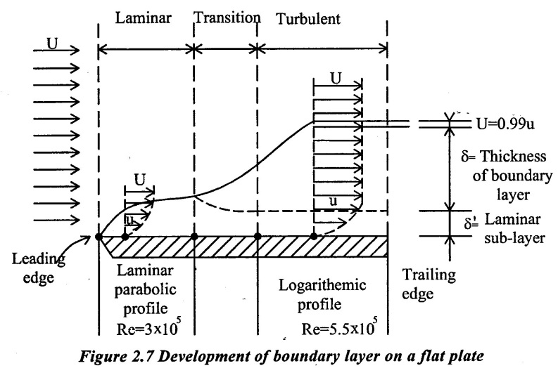
Some of the important characteristics of the boundary layer may be explained by considering a free stream approaching parallel to a sharp edged thin, smooth, flat plat under zero pressure gradient shown in figure 2.7

From the leading edge on wards, the fluid layer immediately adjacent to the boundary attains zero velocity, because of the no slip condition in the region.

1. Factors affecting the growth of boundary layer on a flat plate 

(i) The thickness of the boundary layer grows from leading edge to trailing edge of the plate. More is the distance 'x' from the leading edge, more is this the thickness of the boundary layer.

(ii) Free stream velocity(U): The thickness of boundary layer at any point 'x' from the leading edge is inversely proportional to the free stream velocity. If free stream velocity increases, the thickness of the boundary layer decreases. 

(iii) Density of fluid (ρ): The thickness of boundary layer varies inversely with the density of the fluid. Hence lower density fluids give thicker boundary layer as compared to high density fluids.

(iv) Viscosity of fluids (μ): The boundary layer thickness varies directly proportional to the viscosity of fluids. If viscosity of fluid is high, it will give thicker boundary layer. 

2. Laminar boundary layer

The velocity of fluid on the surface of the plate is equal to velocity of plate and hence is zero since plate is stationary. At a distance away from plate, the fluid has a velocity and thus a velocity gradient is start up near the plate which develop a shear stress which redards fluid. Thus the fluid with a uniform free steam velocity (U) is redard solid surface of the plate.

3. Characteristics of Laminar Boundary layer

(i) It starts from the leading edge of the flat plate.

(ii) The flow in laminar boundary layer consists of one fluid layer moving over adjacent fluid layer. The velocity in Laminar boundary layer varies from zero to the free stream velocity existing out side the layer

(iii) The velocity variation is parabolic

(iv) The thickness of the layer increases with distance 'x' from the leading edge. (v) Newton's law of viscosity is applicable in the Laminar boundary Layer

(vi) It grows up to Reynolds number 3.4 × 105

(vii) The velocity and pressure at a given point are constant with time

4. Transition zone

The length of zone over which the boundary flow changes from laminar to turbulent is called transition zone.

5. Turbulent boundary layer

The thickness of the boundary layer (8) increases with distance from the leading edge. Due to increase the thickness of boundary layer, the laminar boundary layer becomes unstable and motion of fluid is disturbed. This leads to a transition from laminar to Turbulent boundary layer.

6. Characteristics

(i) When Reynolds number is 5 × 105, it starts after the transition boundary layer from the leading edge

(ii) It having a thin laminar sub layer close to the surface of the plate surface 

(iii) The thickness of turbulent boundary layer is more while compare to laminar and transition boundary layer

(iv) The velocity in the boundary layer varies from zero to the main stream velocity outside of the layer

(v) In turbulent boundary layer velocity and pressure at a given point are not constant with time.

(vi) Distribution of velocity varies logarithmically.

7. Laminar sub layer

With in a turbulent boundary layer Zone if the boundary is smooth. A thin layer adjacent to the plate surface over which the flow is assumed to be Laminar is- called Laminar sub-layer. The velocity distribution in the laminar sublayer is Parabolic whereas outside this sublayer in the turbulent boundary layer.

7. Boundary Layer Thickness (δ)

It is defined as the distance from the boundary of the solid body measured in y-direction to the point, where the velocity of the fluid is approximately equal to 0.99 times the free stream velocity (U) of the fluid. It is denoted by (δ) as shown figure 2.8.

1. Types of Boundary Layer thickness

(i) Displacement thickness (δ*)

(ii) Momentum thickness (θ)

(iii) Energy thickness (δ**)

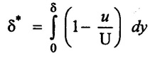
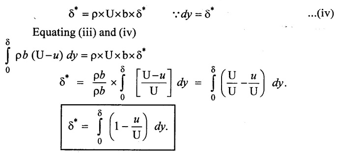
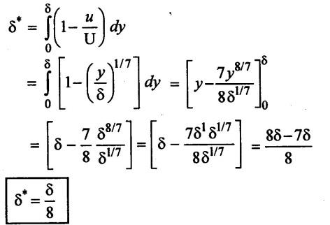
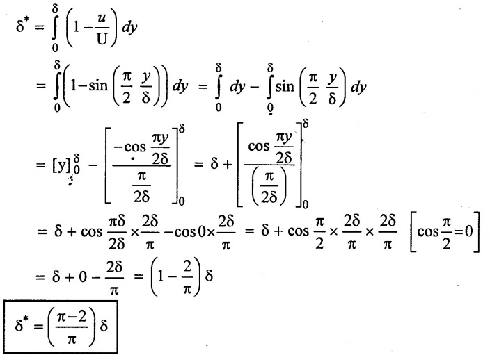
2. Displacement thickness (δ*)

It is defined as the distance measured perpendicular to the boundary of the solid body, by which the boundary should be displaced to compensate for the reduction in discharge in the boundary layer formation. It is denoted by (δ*)

Derivation.

Consider a free stream velocity (U) of flowing fluid over a smooth thin plate as shown in figure 2.9

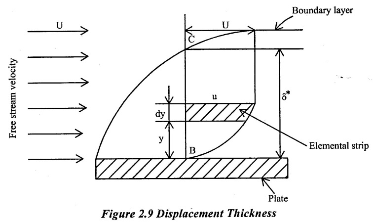
Distance BC = δ*

Velocity varies from zero at B to U at C

Consider a elementary strip at a distance 'y' from the plate and thickness 'dy'

Let 'u' be velocity at elemental strip and 'b' is the width of plate.

⸫ Area of the elemental strip = b × dy

Mass flow rate of fluid/sec flow through elemental strip = Density (ρ) × Discharge (Q)

= ρ × Area of elemental strip × velocity of elemental strip

= ρ × b × dy × u

m = ρ u b dy.        ⸫ m = mass flow rate of fluid/sec

Mass flow rate of fluid/sec flow through elemental strip if no plate is placed (ie) u = U

m = ρ U b.dy             ...(i)

Total reduction of mass flow rate fluid/sec of strip

= ρ U b.dy - ( ρ u b dy)

= ρ.b.dy (U - u)          ...(ii)

Total reduction of mass flow rate of fluid/ sec for whole boundary layer

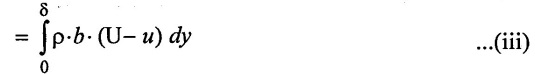
Let the plate displaced by a distance δ* and velocity of flow for the distance δ* is free steam velocity(U).

Loss of Mass flow rate of fluid/sec flowing through distance

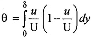
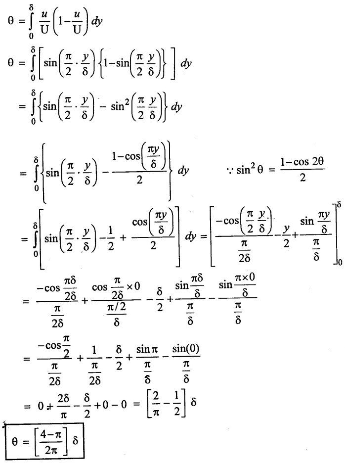
3. Momentum thickness (θ)

Momentum thickness is defined as the distance measured perpendicular to the boundary of the solid body by which the boundary should be displaced to compensate for the reduction in momentum of the flowing fluid in the boundary layer formation. It is denoted by θ.

Derivation:

Consider a free stream velocity (U) of flowing fluid over a smooth thin plate as shown in figure 2.10

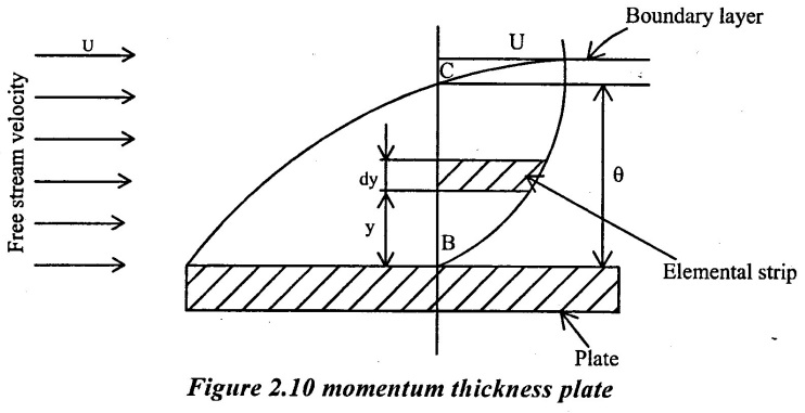Distance BC = θ

Velocity varies from zero at B to U at C

Consider a elementary strip at a distance 'y' from the plate and thickness 'dy'

Let 'u' be the velocity at elemental at strip and 'b' is width of plate.

Area of elemental strip = b × dy

Mass flow rate of fluid/sec, flow through elemental

= Strip Density (ρ) × Discharge(Q)

= ρ × Area of elemental strip × velocity of Elemental strip

= ρ × b × dy × u

m = ρ u b dy.

Momentum of fluid/sec = mass flow rate/sec × velocity

Momentum of fluid/ sec flow through elemental strip

= Mass flow rate/sec × velocity

= ρ u b dy × u

= ρ u2 b dy          ....(i)

Momentum of fluid/sec flow through elemental strip if no plate is placed (u = U).

= ρ u b dy × U   .....(ii)

Loss of momentum/sec through strip

= (ρ u b dy × U) - (ρ u2 b dy)

= ρ⋅b⋅u (U - u) dy   .....(iii)

The total loss of momentum/sec for whole boundary layer BC

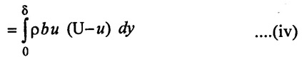
Let θ be distance by which plate is displaced when fluid flowing with constant velocity

Loss of momentum/sec at a distance θ with velocity U = mass of flow through θ × velocity

= (ρ × θ × b × U × U)

= ρ × θ × b × U2   ......(v)

Equating equations (iv) and (v)

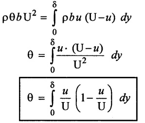
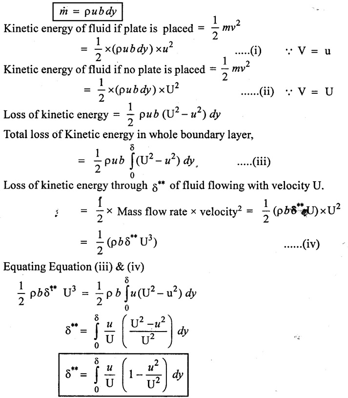
4. Energy thickness (δ**)

It is defined as the distance measured perpendicular to the boundary of the solid body by which the boundary should be displaced to compensate for the reduction in kinetic energy of the flowing fluid in the boundary layer formation. It is denoted by δ**

Derivation:

Consider a free steam velocity (U) of flowing fluid over a smooth thin plate as shown in figure.2.11.

Distance BC = δ**

Velocity varies from zero at B to U at C

Consider a elementary strip at a distance 'Y' from the plate and thickness' dy'

Let 'u' be the velocity at elemental strip and 'b' is width of plate

Area of Elemental stip = b × dy

Mass flow rate of fluid/sec flow through elemental

strip = Density (ρ) × Discharge (Q)

= ρ × Area of elemental strip × velocity of elemental strip

= ρ × b × dy × u 

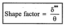
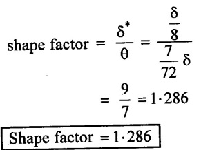
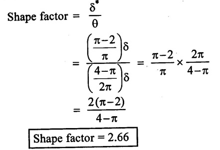
5. Shape factor:

The ratio of displacement thickness (δ**) to momentum thickness (θ) is called as the shape factor

8. Solved Examples based on Boundary Layer Concept 

Example - 18

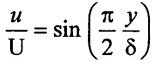
Find the displacement thickness, the momentum thickness and energy thickness for the velocity distribution in the boundary layer given by where u is the velocity at a distance y from the plate and u = U at y = δ, where δ = boundary layer thickness. A so calculate the value of δ*/θ

Solution:

Velocity distribution u/U = y/δ

(i) Displacement thickness (δ*)

(ii) Momentum thickness (θ):

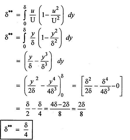
(iii) Energy thickness (δ**)

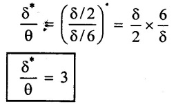
(iv) Shape factor

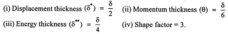
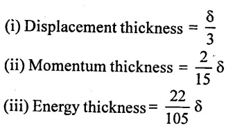
Result:

Example - 19

Find the displacement thickness, momentum thickness, and energy thickness for the velocity distribution in the boundary layer given by.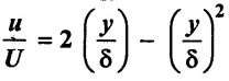

Given:

Solution:

(i) Displacement thickness (δ*)

(ii) Momuntum thickness (θ)

(iii) Energy thickness (δ**)

Result:

Example - 20

The velocity distribution in the boundary layer is given by, 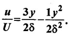Find

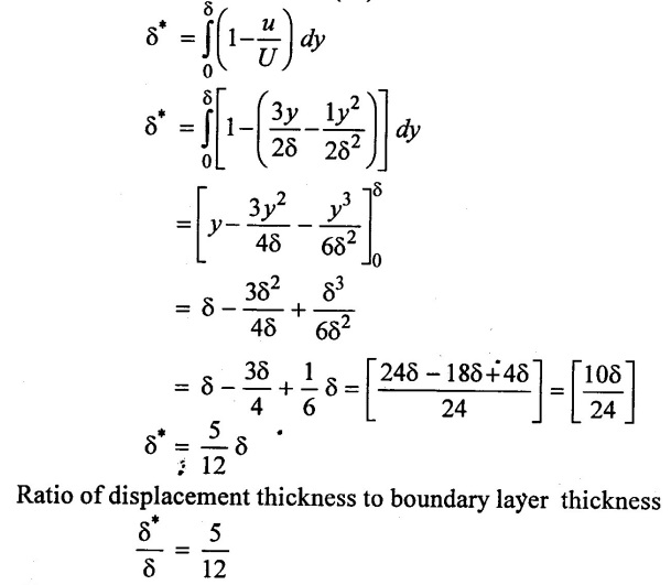
(i) Ratio of displacement thickness to boundary layer thickness

(ii) Ratio of momentum thickness to boundary layer thickness

Given:

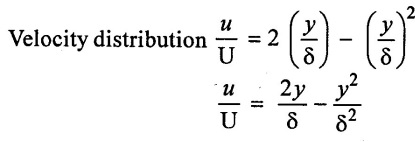
Velocity distribution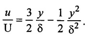

Solution

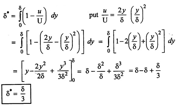
(i) Displacement thickness (δ*)

(ii) Momentum thickness (θ):

Result:

Example - 21

If the velocity distribution in the boundary layer flow over a plate is given by 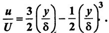Find the displacement thickness where u = velocity of the fluid at any distance y from the plate in a normal direction. U = free stream velocity and δ = boundary layer thickness at any distance × from the leading edge in the direction of flow.

Given:

Solution

Result:

Example - 22

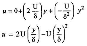
If velocity distribution in laminar boundary layer over a flat plate is assumed to be given by second order polynomical u = a+by+ cy2, determine its form using the necessary boundary condition.

Given

Velocity distribution

u = a + by + cy2

The following boundary condition must be satisfied

Solution

substitute the value of a, b & c in velocity distribution equation.

Result:

Example - 23

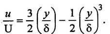
The velocity distribution in the boundary layer is given by calculate

(i) Displacement thickness

(i) Momentum thickness

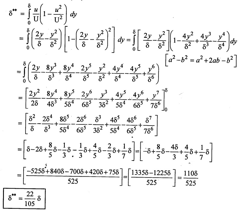
(iii) Energy thickness

(iv) Shape factor

Given

Velocity distribution.

Solution.

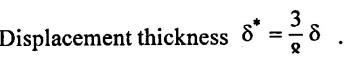
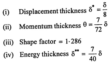
(i) Displacement thickness (δ*)

(ii) Momentum thickness

(iii) Shape factor.

(iv) Energy thickness.

Result:

Example - 24

Velocity distribution in boundary layer is given Find (i) Displacement thickness (ii) Momentum thickness (iii) shape factor

Given:

Velocity distribution.

Solution

(i) Displacement thickness (δ*)

(ii) Momentum thickness (θ)

(iii) Shape factor:

Result:

Example - 25

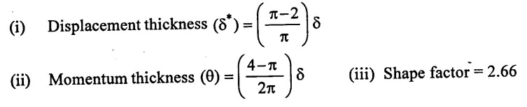
Determine the displacement thickness and momentum thickness in terms of the nominal boundary layer thickness & in respect of the velocity profile in the boundary layer on a plate, Also fluid shape factor if value of m = 3.

Given:

Velocity profile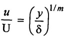

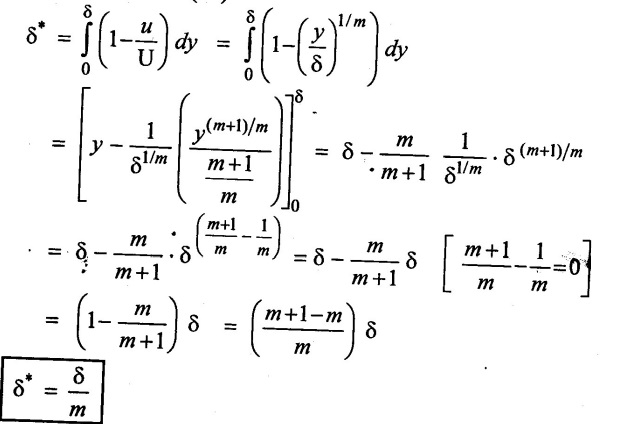
Solution

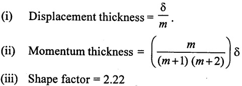
(i) Displacement thickness (δ*)

(ii) Momentum thickness (θ)

(iii) Shape factor.

Result:

9. Momentum Equation for Boundary by Von - Karman (or) Drag Force on Flat Plate due to Boundary Layer.

Consider on flow of a fluid with free stream velocity V over a flat plate as shown in the figure 2.12 consider a small length dx of plate at a distance x from the leading edge of the plate. Now shear near the plate is given by Newton's law of viscosity as

The shear force or drag force acting on dx length of the plate opposite to flow direction is

dFD = Shear stress × Area 

= τo × dx × b          Where b = width.

This drag force dFD has to be equal to the rate of charge of momentum for the flow of fluid on plate for distance dx.

Consider a small control volume PQRS bounded by the boundary surface and boundary layer as shown in figure (b).

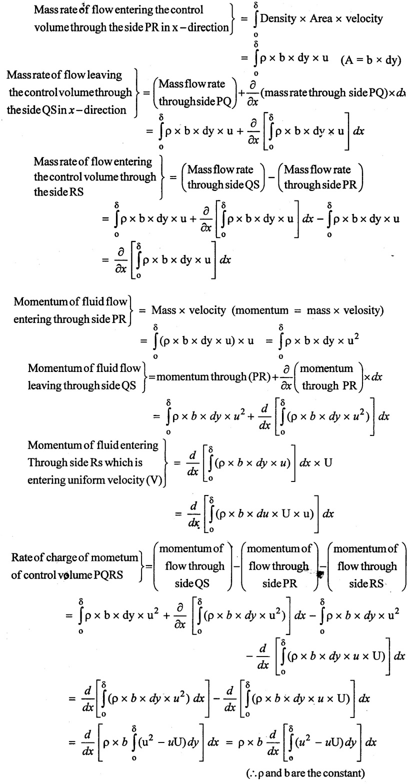
During equilibrium the rate of charge of momentum in control volume (PQRS) is equal to the shear force exerted by the boundary surface on the control volume.

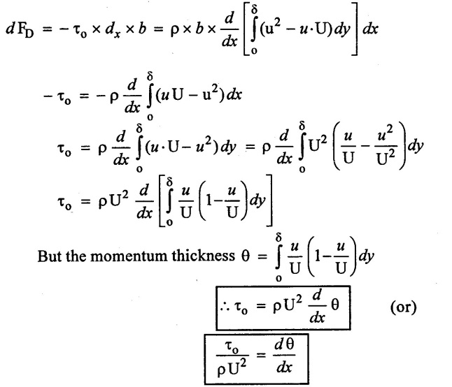
The above equation is known as Von -.Karman momentum equation for boundary layer flow.

10. Boundary Conditions for the Velocity Profiles.

The following are the boundary conditions which must be satisfied by any velocity profile, whether it is in laminar boundary layer zone (or) in turbulent boundary layer zone;

(i) At y = 0, u = 0 and du/dy has same finite value

(ii) At y = δ, u = 0

(iii) At y = δ, du/dy = 0

The shear stress, τo for a given velocity profile in laminar, transition or turbulent zone is obtained. Then,

(i) Drag force on a small distance dx of a plate is given by,

ΔFD shear stress × area

= t。× (b × dx) (assuming width of plate as unity)

= t。× b × dx (where b - width of the plate)

(ii) Total drag on the plate of length L one side,

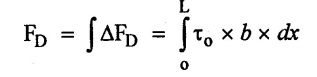
11. Drag Force on Plate (FD)

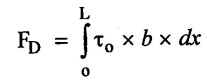
where

το - shear stress

b - width of plate

L - plate length

dx - Distance on plate

12. Local co - Efficient Drag (C*D)

Local co-efficient of drag is defined as ratio of shear stress (τo) to the quantity 1/2 ρV2

Where

V - stream velocity

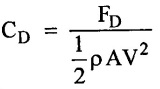
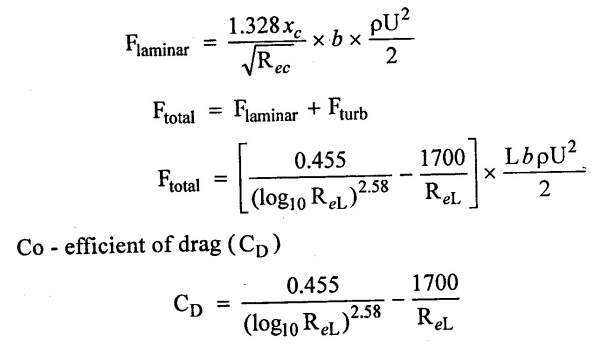
13. Average Co-Efficient of Drag (CD)

Average co - efficient of drag is defined as ratio of total ag force to the quantity ½ ρAV2

14. Drag and Lift Co-Efficient.

Force exerted by a flowing on a stationary body.

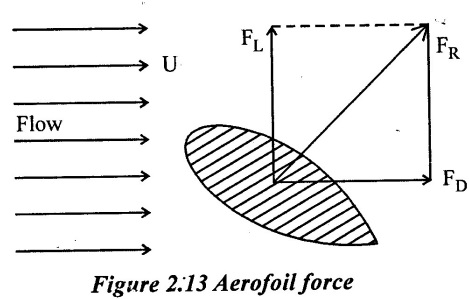
The flowing fluid exerts a force on the stationary body. The total force (FR) is perpendicular to the surface of body. The total force is resolved into two components, first drag force (FD) in the direction of motion, secondly lift force (FL) perpendicular to direction of motion as shown in Figure 2.13

(i) Drag force (FD):-

Component of force in the direction of motion is called drag force. Mathematically,

(ii) Lift force (FL):-

The component of force in the direction perpendicular to the direction of motion is known as lift.

If the axis of the body is parallel to the direction of fluid flow, lift force is zero.

where CD = co-efficient of drag

CL - co-efficient of lift

A = Largest projected area of body.

V = Steam velocity

ρ = density of fluid

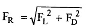
(iii) Total (or) Resultant force on body (FR)

15. Laminar Boundary Layer:

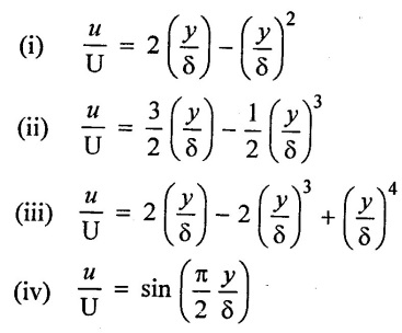
Let us find out boundary layer thickness (δ), shear stress (τ), local co - efficient of drag (C*D) and Average co-efficient of drag (CD) for the following velocity distribution in the laminar boundary layer.

16. Momentum Equation for Turbulent Boundary Layer:

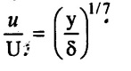
As compared to laminar boundary layers, the turbulent boundary layers are thicker. Further in a turbulent boundary layer the velocity distribution is much more uniform, than in a laminar boundary layer, due to intermingling of fluid particles between different layers of the fluid. The velocity distribution in a turbulent boundary layer follows a logarithmic law i.e. u ∝ log y, which can also be represented by a power law of the type

This known as one-seventh power law.

The above equation cannot be applied at the boundary itself because at y = 0,

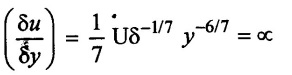
The difficulty is circumvented by considering the velocity in the viscous laminar sublayer to be linear and tangential to the seventh - root profile at the point, where the laminar sublayer merges with the turbulent part of the boundary layer.

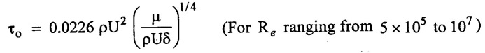
Blasius suggested the following relation for viscous shear stress.

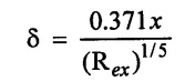
(i) Boundary Layer thickness (δ):

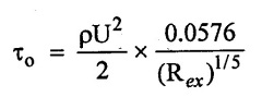
(ii) Shear stress (τ。)

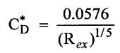
(iii) Local co - efficient of drag (C*D):

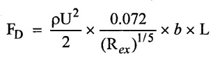
(iv) Drag force (FD):

(vi) Co - efficient (CD):

17. Total Drąg due to Laminar and Turbulent Layers:

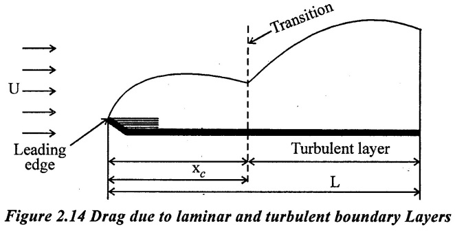
When the leading edge is not very rough, the turbulent boundary layer does not begin at the leading edge it is usually preceded by the laminar boundary layer. The point of transition from laminar or turbulent layer depends upon the intensity of turbulence. The distance xc of the transition from the leading edge can be obtained from critical Reynolds number which normally ranges from 3 × 105 to 3 × 106

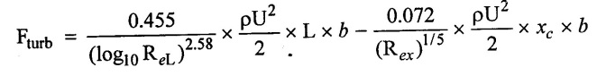
Drag force (FD = F) for the turbulent boundary layer can be estimated from the following relation.

Fturb = (Fturb)total - (Fturb) xc

where

 (Fturb)total = The drag which would occur if a turbulent boundary extends along the entire length if the plate.

(Fturb)xc = The drag due to fictions turbulent boundary layer from the leading edge to a distance xc.

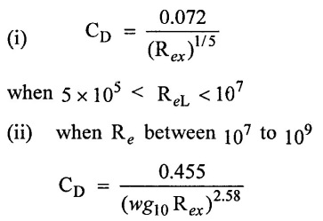
Let us assume that the plate is long enough so that Reynolds number is greater than 107. Then the turbulent drag is given by,

where,

L = Length of the plate

B = width of the plate

U = free stream velocity

The laminar boundary layer prevails with in the length xc and its contribution to drag force is given by

18. Solved Examples based on Laminar and Turbulent Boundary Layer

Example 26

The velocity profile in laminar boundary layer, is Find the thickness of boundary layer at the end and drag force on one side of a plate 2m long and 1.2m wide, when placed in water flowing with a velocity of 0.12 m/ s. Also calculate average co- efficient of drag. Take μ = 0.002 N-s/m2

Given data:

Velocity profile

Length of plate (L) = 2m

wide (or) width (b) = 1.2m

velocity (U) = 0.12 m/s

viscosity (μ) = 0.002 N − s/m2

To find:

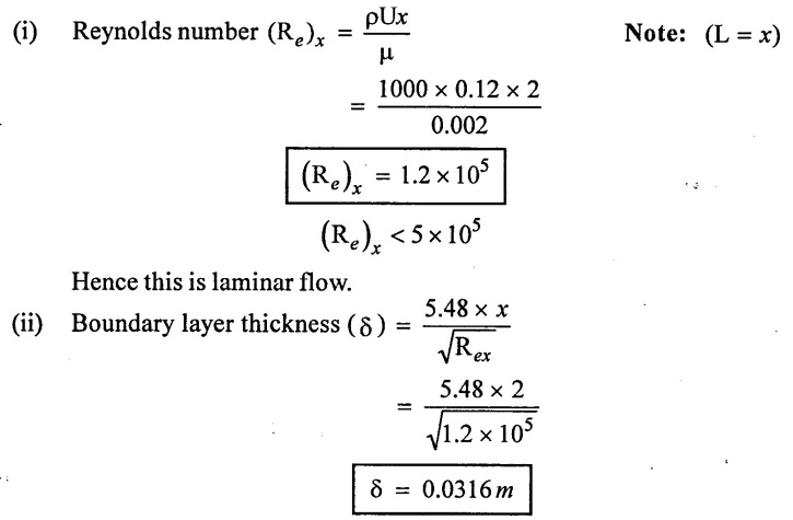
(i) Boundary layer thickness (δ)

(ii) Drag force (FD)

(iii) Average co - efficient of drag (CD)

Solution:

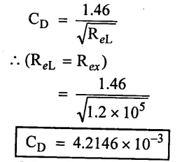
(iii) Average co-efficient of drag (CD)

(iv) Drag force on the side of the plate

Result:

(i) Boundary layer thickness (δ) = 0.0316 m

(ii) Average co-efficient of drag (CD) = 4.2146 × 10−3 

(iii) Drag force (FD) = 0.0728 N

Example - 27

The velocity profile in the form of 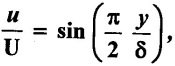Air flows over a plate 0.9m long and 0.6m wide with a velocity of 7 m/s. If density of air 1.24 kg/m3 and kinematic viscosity 0.18 × 10-4 m2/s. Calculate (i) Boundary layer thickness at the end of the plate (ii) shear stress at 300mm from the leading edge and (iii) Drag on one side of the plate.

Given data:

Velocity profile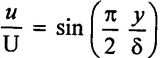

Length (L) = 0.9m

wide (w) (or) (b) = 0.6m 

velocity (U) = 7 m/s

Density (ρ) = 1.24 kg / m3

Kinematic viscosity (v) = 0.18 × 10-4 m2/s

To find: 

(i) Boundary layer thickness at x = L

(ii) shear stresses at x = 300mm 

(iii) Drag force (FD)

Solution:

Result

(i) Boundary layer thickness (δ) = 7.294 × 10-3 m

(ii) shear stress (τo) = 0.058 N/m2

(iii) Drag force (FD) = 0.03632 N

Example - 28

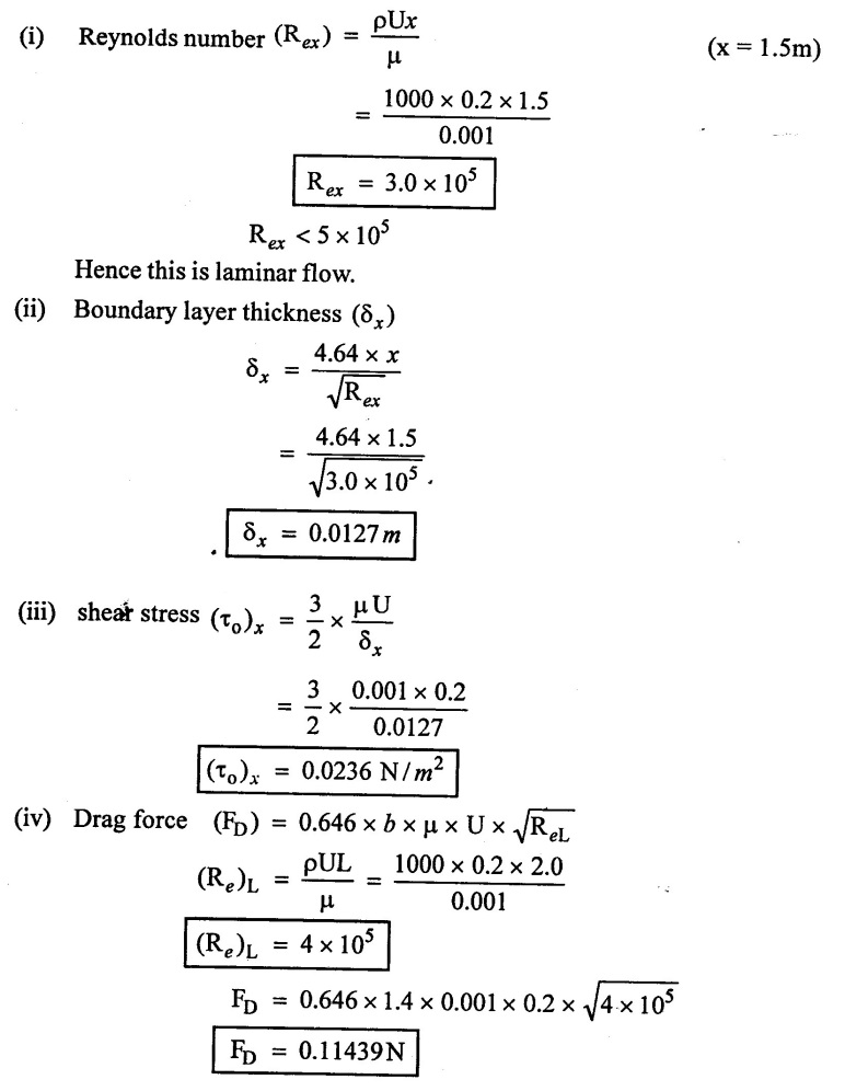
For the velocity profile in laminar boundary layer as 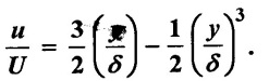Find the thickness of the boundary layer and the shear stress 1.5m from the leading edge of a plate. The plate is 2m long and 1.4m wide and placed in water which is moving with a velocity of 200mm per second. Find the total drag force on the plate if μ for water = 0.01 poise.

Given data:

velocity profile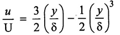

Local distance (x) = 1.5m

Length of plate (L) = 2m

width of plate (w) (or) (b) = 1.4m

Velocity of plate (U) = 200 mm/s = 0.2 m/s

viscosity (μ) = 0.01 poise = 0.001 N-s/m2

To find:

(i) Boundary layer thickness at x = 1.5m

(ii) shear stress at x = 1.5m

(iii) Total drag force on both side of the plate

Solution:

Result

(i) Boundary layer thickness (δx) = 0.00127 m

(ii) shear stress (τo)x = 0.0236 N/m2

(iii) Drag force (FD) = 0.11439 N

Example 29

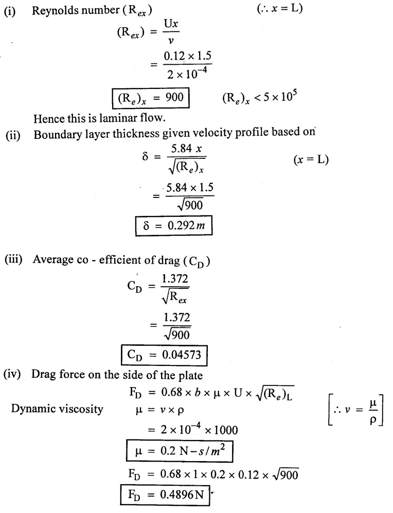
For the velocity profile in laminar boundary layer as 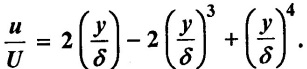Find the thickness of the boundary layer at the end and drag force on one side of a plate 1.5m long and 1m wide. when placed in water flowing with a velocity of 0.12 m/s. Also calculate coefficient of drag. Take v = 2 × 10-4 m3/s

Given data:

Velocity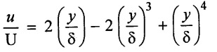

Length of plate (L) = 1.5 m

wide (or) width (w) = 1m 

velocity (U) = 0.12 m/s

kinematic viscosity (v) = 2 × 10-4 m3 / s

To find:

(i) Thickness of boundary layer (δ)

(ii) Drag force on the side of plate (FD) 

(iii) Average co-efficient of drag (CD)

Solution:

Result:

(i) Boundary layer thickness (δ) = 0.292 m

(ii) Average co-efficient of drag (CD) = 0.04573

(iii) Drag force on the side of the plate (FD) = 0.4896 N

Example - 30

A thin plate is moving still atmospheric air at a velocity of 4 m/s. The length of the plate is 1.4 m and width 0.7m. Calculate thickness of the boundary layer at the end of the plate and Drag force on both side of the plate. Take density of air is 1.24 kg/m3 and kinematic viscosity 0.15 stokes.

Given data:

velocity of the plate (U) = 4 m/s 

Length of the plate (L) = 1.4 m

width of the plate (w) = 0.7 m

Density of air (ρ) = 1.24 kg/m3

kinematic viscosity (v) = 0.15 stokes = 0.15 × 10-4 m2/s

To find:

(i) Boundary layer thickness δ at x = L

(ii) Total drag force (FD)

Solution:

Here any velocity profile is not given so that Blasius solution will be used.

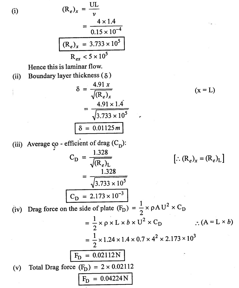
Result:

(i) Boundary layer thickness (δ) = 0.01125 m

(ii) Total drag force (FD) = 0.04224 N.

Example - 31

A plate of 800mm length and 500mm wide is immersed in a fluid of specific gravity 0.8 and dynamic viscosity 0.002 N-s/m2. The fluid moving with a velocity of 4 m/s. Determine the (i) boundary layer thickness at end of plate (ii) shear stress at the end of plate (iii) drag force one side of the plate.

Given data:

Length of plate (L) = 800 mm = 0.8m

width of plate (w) = 500 mm = 0.5m

specific gravity of fluid = 0.8

Dynamic viscosity (μ) = 0.002 N - s/m2

velocity of fluid (U) = 0.4 m/s

To find:

(i) Boundary layer thickness at end of the plate (δ)

(ii) shear stress at end of the plate (τo)

(iii) Drag force on the side of the plate (FD)

Solution:

This problem is not mention any velocity profile. So that Blasiuss solution will be used.

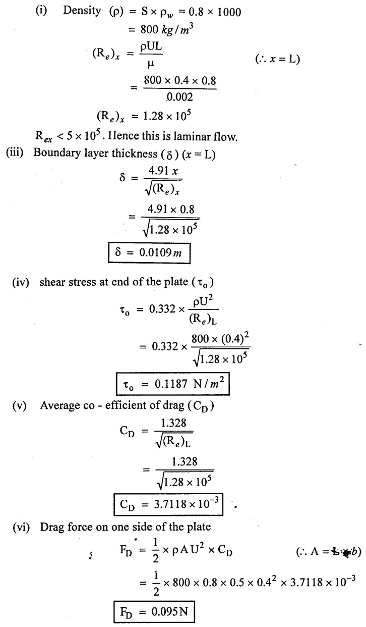
Result:

(i) Boundary Layer thickness (δ) = 0.0109 m

(ii) shear stress (τo) = 0.1187 N/m2

(iii) Drag force on one side (FD) = 0.095N

Example - 32

Air at 25°c and 1 bar flows over a flat plate at a speed of 1.25 m/s. Calculate the boundary layer thickness at distance of 20 cm and 30cm from the leading edge of the plate. What would be the mass entrainment (or) entering between these two sections? Assume parabolic velocity distribution is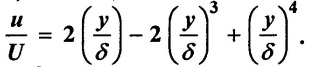

The viscosity of air at 25°c is stated to be 6.62 × 10+ kg/hr - m

[1 Pa.s = 1 Ns/m2 = 1 kg/ms]

Given data:

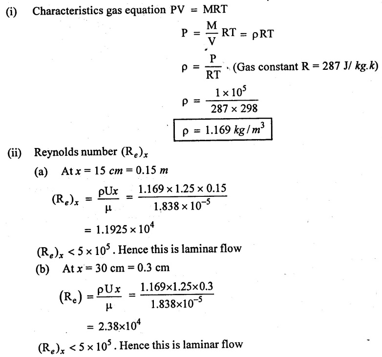
Temperature (T) 25°c + 273 = 298k

Pressure (P) = 1 bar = 1 × 105 N/m2

velocity (U) = 1.25 m/s

Dynamic viscosity (μ) = 6.62 × 10-2 kg/hr-m =

= 1.838 × 105 kg/sm

= 1.838 × 10-5 N-s/m2

To find: 

(i) Boundary layer thickness at x = 20 cm & x = 30cm 

(ii) Mass flow rate between two sections.

Note:

[⸫ 1N - s/m2 = 1 kg/m-s]

Solution:

(iii) Boundary layer thickness based on given velocity profile 

(a) Boundary layer thickness (δ) at x = 0.15 m

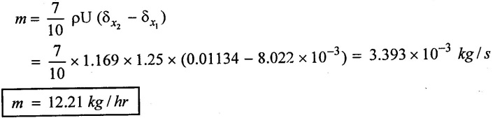
(v) mass entering between two sections

Result:

(i) Boundary layer thickness (δx1) at x = 0.15m = 8.022 × 10-3 m 

(ii) Boundary layer thickness (δx2) = at x = 0.3 m = 0.01134m 

(iii) mass entering between two sections (m) = 12.21 kg/hr

Example - 33

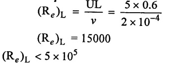
A plate 0.6m × 0.3m has been placed longitudinally in a steam of crude oil which flows with undisturbed velocity 5 m/s. given that of oil has a specific gravity 0.9 and kinematic viscosity 2 stokes. Calculate the boundary layer thickness and shear at the middle of the plate. Also calculate friction drag on one side of the plate. 

Given data:

Size of plate = 0.6 × 0.2m

velocity (U) = 5 m/s

specific gravity (s) = 0.9

kinematic viscosity (v) = 2 stoke = 2 × 10-4 m2/sec

To find:

(i) Boundary layer thickness at middle of the plate (δx)

(ii) shear stress at middle of the plate (τo)x

(iii) Friction drag one side of the plate (CD)

Solution:

This problem is not given any velocity profile. So that Blasiuss solution will be used.

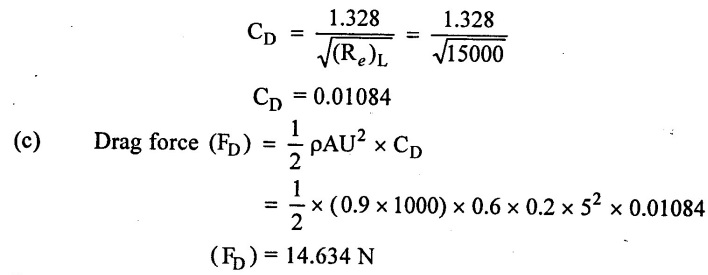
(v) frictional drag force on one side of the plate (x = 0.6)

(b) Average frictional drag based on Blasiuss solution

Result:

Boundary layer thickness (δ)x = 0.0173 m

shear stress (τo)x = 86.25 N/m2

Drag force (FD)x=0.6 = 14.634 N

Example - 34

A smooth plate of length 5m and width of 1.6m when the plate moving with a velocity of 5 m/s in stationary air. Kinematic viscosity and density of air are 1.5 × 10-5 m2/s and 1.226 kg/m3 respectively. Find the boundary layer thickness of end of the plate and the total drag on one side of the plate assuming that (i) boundary layer is laminar over the entire length (ii) the boundary is turbulent from the very begining. 

Given data:

Length of plate (L) = 5m

width of plate (w) = 1.6m 

Velocity (U)= 5 m/s

kinematic viscosity (v) 1.5 × 10-5 m2 / s

Density (ρ) = 1.226 kg/m3

To find:

(i) Boundary Layer thickness to entire length

(ii) Drag force (FD) when entire length of boundary layer is laminar 

(iii) Drag force (FD) when entire length of boundary layer is turbulent.

Solution:

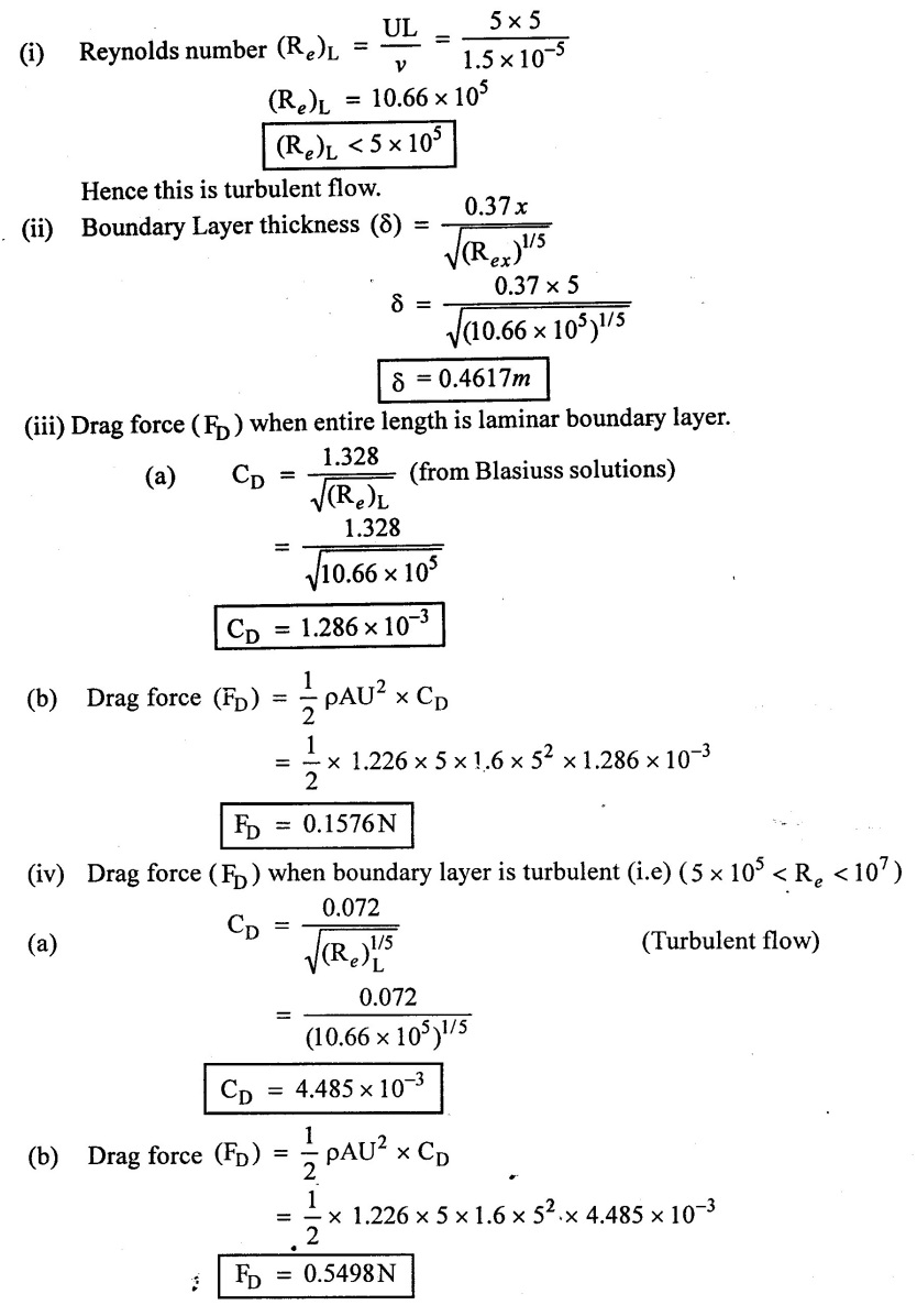
Result:

(i) Boundary Layer thickness (δ) = 0.4617m

(ii) Drag force (FD) when Laminar = 0.1576N

(iii) Drag force (FD) when Turbulent = 0.5498N.

Example - 35

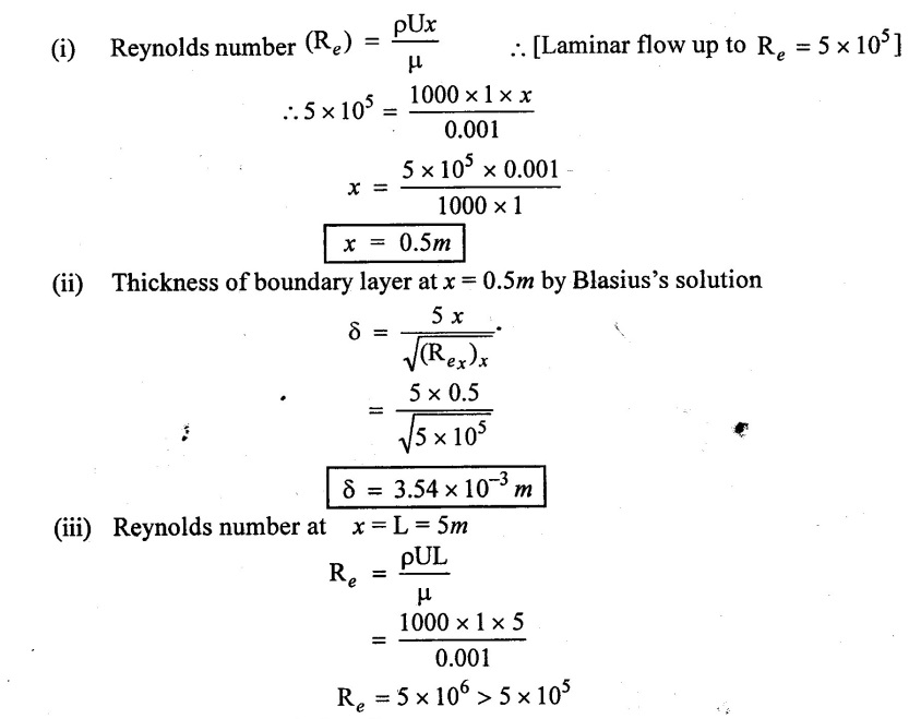
A plate 5m × 3m is held in water moving at 1 m/s parallel to its length. If the Flow is the boundary layer is Laminar at the leading edge of the plate. Determine 

(i) Distance from the leading edge where the boundary layer changes from laminar to turbulent.

(ii) Thickness of boundary layer at this section

(iii) The drag force on one side of the plate. Take μ = 0.001 pa.s.

Given data:

Length (L) = 5m

width (b) = 3m

velocity (U) = 1 m/s

viscosity (μ) = 0.001 pa.s = 0.001 N-s/m2

To find: 

(i) Distance from leading edge to the point where boundary layer changes from laminar to turbulent.

(ii) Boundary layer thickness at transition zone

(iii) The drag force on one side of the plate.

Solution:

Hence this is Turbulent flow.

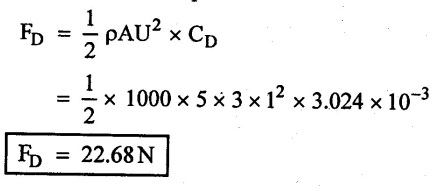
(iv) Average co-efficient of Drag in partly laminar partly turbulent flow.

(v) Drag force on one side of the plate.

Result:

(i) Laminar flow distance (x) = 0.5m

(ii) Laminar flow boundary layer thickness (δ) 3.54 × 10-3 m

(iii) The drag force both mixed flow on one side of the plate FD = 22.68 N 

19. Boundary Layer Separation.

Flow generally takes place from higher pressure to lower pressure which is called negative pressure gradient (i,e) pressure is decreasing in the direction of flow or pressure gradient in x - direction is However, there are situations when flow takes place over a curved boundary surface under positive pressure gradient (i.e) pressure is increasing in the direction of the flow.

In such cases, the flow near the boundary is continuously retarded and a point is reached when the flow starts separating from the boundary. The point at which flow separates from the boundary is called separation point. The separation takes place mainly due to positive pressure gradient which reduces the momentum of flow of the fluid within the boundary layer due to higher shear stresses in fluid having high viscosity. The change of velocity and pressure gradient are related as -

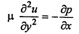
The flow accelerates or velocity increases in case is negative. The flow deaccelerates or velocity decreases if is positive.

1. Effect of Boundary layer separation.

Consider a flow over a curved surface causing positive pressure gradient (i.e) is positive as shown in figure 2.15 the flow starts retarding as it moves forward from point (1) the flow velocity gradually diminishes to zero at point (2). The fluid particles cannot move further close to boundary surface as these particles have to encounter the resistance of the boundary layer. Hence fluid leaves the boundary at point(2).

The separation gap increases as the fluid moves beyond point (2) to (3). The layer of fluid detached from point (2) has tendency to roll it self, there by forming vortices. This region where vortices are formed due to positive pressure gradient is called wake. The kinetic energy of the flow is wasted due to reverse flow which is ultimately converted into internal energy (increase the temperature of the fluid). There is additional drag force in the wake ration. The velocity distribution helps in identification of separation as under-

The positive velocity gradient leads to reduction in the velocity in the boundary. layer. Reynolds number decreases with velocity retardation. Since the thickness of the boundary layer is inversely proportional to boundary layer increases with positive pressure gradient.

2. Methods of preventing the separation of boundary Layer.

The separation of boundary layer is undesirable and attempts are made to avoid separation by various methods. The methods for preventing the separation of boundary layer are.

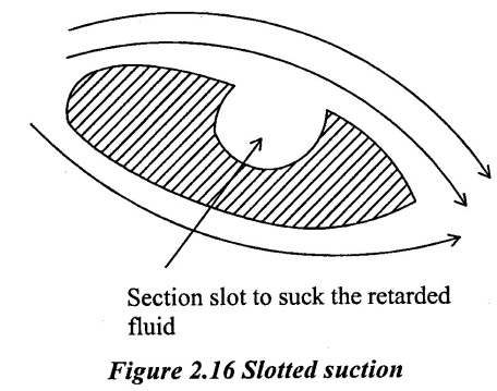
(i) Suction of slow moving fluid by a suction slot.

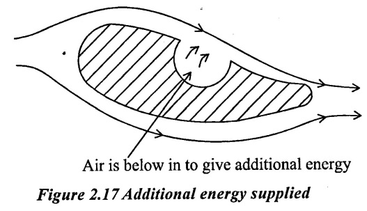
(ii) Supplying additional energy from a blower

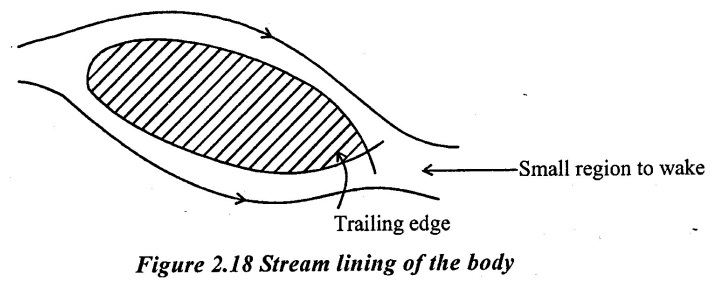
(iii) Streamlining of the body so that separation is avoided or take place as near to the trailing edge

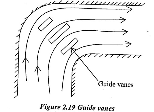
(iv) Providing guide vanes to guide fluid to avoid separation

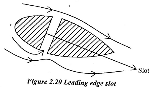
(v) Providing slot near the leading edge